OpenTelemetry has revolutionized the observability landscape by liberating us from vendor lock-in. It empowers us to collect our data and seamlessly transition between platforms, breaking free from the constraints of proprietary solutions.

Traditional observability setups can be prohibitively costly. How can we build an observability solution without breaking the bank? Enter Feldera. Feldera is an open-source platform that is easy to deploy yourself. In Feldera, everything is defined using SQL, allowing engineers familiar with SQL to be instantly productive without the need to learn proprietary languages.

At its core, OpenTelemetry data consists of a continuous stream of append-only records containing logs, metrics, and traces. This type of workload is perfectly suited for Feldera's incremental computation engine, which efficiently processes and analyzes this data in real-time.

By the end of this article, we aim to build a comprehensive observability dashboard for analyzing OTel data.

Grafana Dashboard visualizing Feldera generated insights from OpenTelemetry data.

This dashboard takes inspiration from the workshop: Analyzing and Visualizing OpenTelemetry Traces with SQL - John Pruitt, Timescale

The source code for this OpenTelemetry Demo is available in feldera/otel-demo.

Architecture

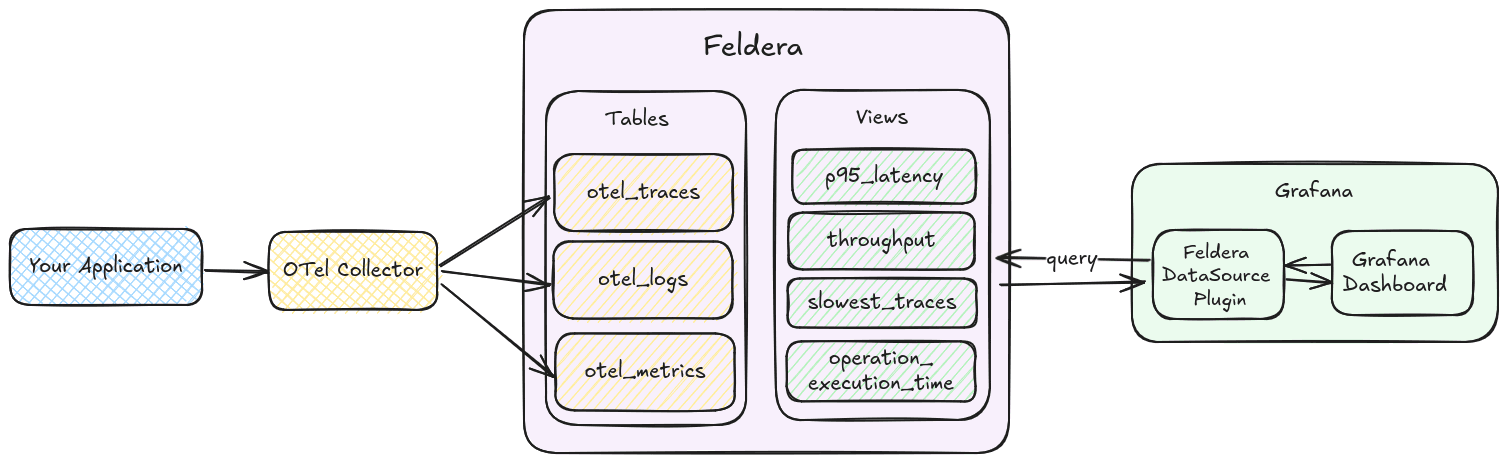
We use the OpenTelemetry Demo application to generate data, which is collected by the OTel Collector and sent to respective Feldera tables. We then define views on this data and use the Feldera plugin for Grafana to make ad-hoc queries to Feldera and visualize the results as a dashboard.

This setup demonstrates how Feldera can be used for observability workloads, but its capabilities extend far beyond this use case.

Representing OTel Data

OTel data consists of nested JSON, which we model as user-defined SQL types in Feldera based on the OTel Protobuf definitions.

CREATE TYPE KeyValue AS (
    key VARCHAR,
    value VARIANT
);

CREATE TYPE Event AS (
    timeUnixNano CHAR(20),
    name VARCHAR,
    attributes KeyValue ARRAY
);

CREATE TYPE Span AS (
    traceId VARCHAR,
    spanId VARCHAR,
    traceState VARCHAR,
    parentSpanId VARCHAR,
    flags BIGINT,
    name VARCHAR,
    kind INT,
    startTimeUnixNano CHAR(20),
    endTimeUnixNano CHAR(20),
    attributes KeyValue ARRAY,
    events Event ARRAY
);

CREATE TYPE Metric AS (
    name VARCHAR,
    description VARCHAR,
    unit VARCHAR,
    sum VARIANT,
    gauge VARIANT,
    summary VARIANT,
    histogram VARIANT,
    exponentialHistogram VARIANT,
    metadata KeyValue ARRAY
);

CREATE TYPE LogRecords AS (
    attributes KeyValue ARRAY,
    timeUnixNano CHAR(20),
    observedTimeUnixNano CHAR(20),
    severityNumber INT,
    severityText VARCHAR,
    flags INT4,
    traceId VARCHAR,
    spanId VARCHAR,
    eventName VARCHAR,
    body VARIANT
);

CREATE TYPE Scope AS (
    name VARCHAR,
    version VARCHAR,
    attributes KeyValue ARRAY
);

CREATE TYPE ScopeSpans AS (
    scope Scope,
    spans Span ARRAY
);

CREATE TYPE ScopeLogs AS (
    scope Scope,
    logRecords LogRecords ARRAY
);

CREATE TYPE ScopeMetrics AS (
    scope Scope,
    metrics Metric ARRAY
);

CREATE TYPE Resource AS (
    attributes KeyValue ARRAY
);

CREATE TYPE ResourceMetrics AS (
    resource Resource,
    scopeMetrics ScopeMetrics ARRAY
);

CREATE TYPE ResourceSpans AS (
    resource Resource,
    scopeSpans ScopeSpans ARRAY
);

CREATE TYPE ResourceLogs AS (
    resource Resource,
    scopeLogs ScopeLogs ARRAY
);

The following graph illustrates the type hierarchy of the custom types defined above:

Diagram that represents the type hierarchy of OTel data in Feldera SQL.

Note that value in the type KeyValue is of type VARIANT. VARIANT is designed to be used for dynamically typed values and JSON objects. (VARIANT docs)

Now that we have the type definitions to represent the OTel data, we create tables. Tables in Feldera model input data streams.

-- Input table that ingests resource spans from the collector.
CREATE TABLE otel_traces (
    resourceSpans ResourceSpans ARRAY
) WITH ('append_only' = 'true');

-- Input table that ingests resource logs from the collector.
CREATE TABLE otel_logs (
    resourceLogs ResourceLogs ARRAY
) WITH ('append_only' = 'true');

-- Input table that ingests resource metrics from the collector.
CREATE TABLE otel_metrics (
    resourceMetrics ResourceMetrics ARRAY
) WITH ('append_only' = 'true');

Feldera operates on changes, so any input may be an insertion or deletion. Setting 'append_only' = 'true' allows Feldera to potentially optimize the programs better and ensures only insertions are supported for this table.

Sending OTel data to Feldera

Feldera can accept data from multiple sources. Typically, you configure a connector to allow Feldera to fetch data from a source or send it to a sink (see Connectors Docs). However, you can also push data directly to a Feldera table with HTTP.

To push data to a Feldera table via HTTP, you make a POST request to:

http://{FELDERA_HOST}/v0/pipelines/{PIPELINE_NAME}/ingress/{TABLE_NAME}

We configure the OTel collector to export all traces, logs and metrics to Feldera by modifying src/otel-collector/otelcol-config-extras.yml.

# src/otel-collector/otelcol-config-extras.yml in OpenTelemetry Demo

exporters:

  # Send traces to the Feldera pipeline.
  # Currently only uncompressed JSON is supported.
  otlphttp/feldera:
     logs_endpoint: http://feldera:8080/v0/pipelines/otel/ingress/otel_logs?format=json&update_format=raw
     traces_endpoint: http://feldera:8080/v0/pipelines/otel/ingress/otel_traces?format=json&update_format=raw
     metrics_endpoint: http://feldera:8080/v0/pipelines/otel/ingress/otel_metrics?format=json&update_format=raw
     encoding: json
     compression: none

service:
   pipelines:
     traces:
       receivers: [otlp]
       processors: [transform, batch]
       exporters: [spanmetrics, otlphttp/feldera, debug, otlp]

     logs:
       receivers: [otlp]
       processors: [batch]
       exporters: [otlphttp/feldera, debug]

     metrics:
       receivers: [hostmetrics, docker_stats, httpcheck/frontend-proxy, otlp, prometheus, redis, spanmetrics]
       processors: [batch]
       exporters: [otlphttp/feldera, debug]

Notice that we have the query parameters: format=json&update_format=raw

format=json: Specifies that the input data is JSON-formatted.
update_format=raw: Indicates that the request body contains raw data, which Feldera processes as an insertion into the table.

Pre-processing

The OTel data format contains data in arrays of fields, we want to convert them into traditional database table rows, this would allow for easier processing in SQL.We do this by performing a series of UNNEST operations.

Step 1: Extract Resource-Level Data

-- concat with the previous table definitions

-- (ResouceMetrics[N]) -> (Resource, ScopeMetrics[N])
CREATE LOCAL VIEW rsMetrics AS SELECT resource, scopeMetrics
FROM otel_metrics, UNNEST(resourceMetrics) as t (resource, scopeMetrics);

-- (ResouceSpans[N]) -> (Resource, ScopeSpans[N])
CREATE LOCAL VIEW rsSpans AS SELECT resource, scopeSpans
FROM otel_traces, UNNEST(resourceSpans) as t (resource, scopeSpans);

-- (ResouceLogs[N]) -> (Resource, ScopeLogs[N])
CREATE LOCAL VIEW rsLogs AS SELECT resource, scopeLogs
FROM otel_logs, UNNEST(resourceLogs) as t (resource, scopeLogs);

Here we UNNEST arrays of ResourceSpans, ResourceMetrics and ResourceLogs into separate rows.

Step 2: Extract Scope-Level Data

-- (ScopeMetrics[N]) -> (ScopeMetrics) x N
CREATE LOCAL VIEW metrics_array AS
SELECT
    resource,
    scope,
    metrics
FROM rsMetrics, UNNEST(rsMetrics.scopeMetrics) as t(scope, metrics);

-- (ScopeLogs[N]) -> (ScopeLogs) x N
CREATE LOCAL VIEW logs_array AS
SELECT
    resource,
    scope,
    logs
FROM rsLogs, UNNEST(rsLogs.scopeLogs) as t(scope, logs);

-- (ScopeSpans[N]) -> (ScopeSpans) x N
CREATE LOCAL VIEW spans_array AS
SELECT
    resource,
    scope,
    spans
FROM rsSpans, UNNEST(rsSpans.scopeSpans) as t(scope, spans);

Similarly, we UNNEST the ScopeMetrics, ScopeLogs and ScopeSpans into separate rows.

Step 3: Extract Final Metrics and Logs

-- (Metrics[N]) -> (_, Metric) x N
CREATE MATERIALIZED VIEW metrics AS
SELECT
    name,
    description,
    unit,
    sum,
    summary,
    gauge,
    histogram,
    exponentialHistogram,
    resource,
    scope,
    metadata
FROM metrics_array, UNNEST(metrics_array.metrics);

-- (Logs[N]) -> (_, Logs) x N
CREATE MATERIALIZED VIEW logs AS
SELECT
    resource,
    scope,
    attributes,
    timeUnixNano,
    observedTimeUnixNano,
    severityNumber,
    severityText,
    flags,
    traceId,
    spanId,
    eventName,
    body
FROM logs_array, UNNEST(logs_array.logs);

Finally, we extract individual Metric and LogRecords to extract individual records.

Step 4: Process Spans and Add Derived Fields

For spans, we not only extract individual records but also compute useful derived fields:

elapsedTimeMillis: The duration of the span in milliseconds.
eventTime: Timestamp for when the span started. Note that in Feldera, the TIMESTAMP type doesn't include time zone information.

-- Convert nanoseconds to seconds
CREATE FUNCTION NANOS_TO_SECONDS(NANOS BIGINT) RETURNS BIGINT AS
(NANOS / 1000000000::BIGINT);

-- Convert nanoseconds to milliseconds
CREATE FUNCTION NANOS_TO_MILLIS(NANOS BIGINT) RETURNS BIGINT AS
(NANOS / 1000000::BIGINT);

-- Convert to TIMESTAMP type from a BIGINT that represents time in nanoseconds
CREATE FUNCTION MAKE_TIMESTAMP_FROM_NANOS(NANOS BIGINT) RETURNS TIMESTAMP AS
TIMESTAMPADD(SECOND, NANOS_TO_SECONDS(NANOS), DATE '1970-01-01');

-- (Spans[N]) -> (Span, elapsedTimeMillis, eventTime) x N
CREATE MATERIALIZED VIEW spans AS
SELECT
    resource,
    scope,
    traceId,
    spanId,
    tracestate,
    parentSpanId,
    flags,
    name,
    kind,
    startTimeUnixNano,
    endTimeUnixNano,
    attributes,
    events,
    NANOS_TO_MILLIS(endTimeUnixNano::BIGINT - startTimeUnixNano::BIGINT) as elapsedTimeMillis,
    MAKE_TIMESTAMP_FROM_NANOS(startTimeUnixNano) as eventTime
FROM spans_array, UNNEST(spans_array.spans);

Here we leverage SQL based user defined functions (UDFs) to define functions that may come in handy later.

Extracting High-Level Metrics

In this blog, we will focus on calculating the P95 latency to demonstrate how to extract high-level metrics from OpenTelemetry data. For more detailed metrics and a comprehensive guide, please refer to the full documentation: Use Case: OpenTelemetry.

P95 Latency

P95 latency is a common statistical measure used for network performance analysis. It means that 95% of requests were served faster than this value, while 5% took longer than this.

Step 1: Define a Tumbling Window

To compute P95 latency over time, we first define a 10-second tumbling window on the spans view. This might be useful later on for other insights as well!

-- continuation of the SQL program

CREATE LOCAL VIEW spans_tumble_10s AS
SELECT * FROM TABLE(
	TUMBLE(
		TABLE spans,
		DESCRIPTOR(eventTime),
		INTERVAL '10' SECOND
	)
);

This groups spans into non-overlapping 10-second time windows.

Step 2: Define a Rust UDF for P95 Calculation

Calculating the P95 value in SQL might not be trivial. Here we leverage Feldera's support for Rust UDFs.

SQL Definition for P95 Rust UDF

-- UDF to calculate p95 value given an integer array
CREATE FUNCTION p95(x BIGINT ARRAY NOT NULL) RETURNS BIGINT;

Rust Implementation of P95

// udf.rs

pub fn p95(x: Vec<Option<i64>>) -> Result<Option<i64>, Box<dyn std::error::Error>> {
	let mut x: Vec<i64> = x.into_iter().filter_map(|x| x).collect();

	if x.is_empty() {
		return Ok(None);
	}

	x.sort_unstable();

	let rank = 0.95 * x.len() as f64 - 1.0;
	let lower = rank.floor() as usize;
	let upper = rank.ceil() as usize;

	if lower == upper {
		Ok(Some(x[lower]))
	} else {
		let weight = rank - lower as f64;
		Ok(Some((x[lower] as f64 * (1.0 - weight) + x[upper] as f64 * weight) as i64))
	}
}

This function:

Filters out null values and sorts the values.
Finds the 95th percentile index.
Interpolates and returns the P95 value.

Step 3: Compute P95 Latency per 10 Second Window

-- Calculate the p95 latency in milliseconds
CREATE MATERIALIZED VIEW p95_latency AS
SELECT
	p95(array_agg(elapsedTimeMillis)) as latencyMs,
	window_start as 'time'
FROM spans_tumble_10s
WHERE
	parentSpanId = '' -- Only consider top-level requests
GROUP BY
	window_start;

This filters only the top level traces and aggregates elapsedTimeMillis values into an array and calls the p95 function.

Grafana Integration

Step 1: Install the Feldera Grafana Plugin

Since the Feldera datasource plugin is not yet available in the Grafana marketplace, it must be manually installed from GitHub. You can download the latest release and unzip in in the plugins directory of your Grafana server.

Step 2: Add Feldera as a Data Source in Grafana
Steps to add a new data source:

Open the Grafana Dashboard and go to Connections -> Add New Connection
Search for Feldera and select the Feldera Data Source Plugin.
Click Add a new data source.

Step 3: Configure the Feldera Data Source

Feldera Data Source Configuration in Grafana

Required Fields:

Field	Value
Base URL	http://feldera:8080 (If running in Docker alongside Grafana)
Pipeline Name	otel (Your Feldera pipeline name)
API Key	(If authentication is required, provide the API Key)

Click Save & Test to verify the connection.

Creating a Grafana Dashboard

Once Feldera is set up as a data source, you can build a custom Grafana dashboard to visualize OpenTelemetry data.

For all the visualizations we create here, use the feldera data source.

Requests Count

This visualization displays the total number of requests in the selected time range.
Visualization Type: Stat

-- requests count
SELECT 
	COUNT(*) as num_traces 
FROM 
	spans s
WHERE 
	s.parentSpanId = '' AND 
	s.eventTime BETWEEN $__timeFrom() AND $__timeTo()

Filters only top-level spans (i.e., spans without a parentSpanId).

Uses Grafana's $__timeFrom() and $__timeTo() macros to dynamically apply the selected time range.

P95 Latencies

Tracks the 95th percentile latency over time.
Visualization Type: Bar chart

-- p95_latency
SELECT 
	* 
FROM 
	p95_latency 
WHERE 
	time BETWEEN $__timeFrom() AND $__timeTo() 
ORDER BY 
	time DESC

Conclusion

Telemetry data is often massive in scale, yet it's absolutely crucial for cloud observability. Instead of setting up a complex observability stack or relying on expensive vendor solutions, Feldera offers a lightweight, open-source way to analyze telemetry data using plain SQL.

In this article, we walked through the process of ingesting raw OpenTelemetry data into Feldera tables and leveraging SQL to extract key performance insights. We then demonstrated how effortlessly this data can be queried in Grafana, creating an observability solution with minimal setup. While Grafana serves as a simple demonstration, these insights can be streamed to various other sinks for broader integration.

Whether you're troubleshooting slow requests, analyzing system performance, or tracking request volume, Feldera provides a scalable, SQL-first approach to telemetry. Two key features make it particularly well-suited for observability:

Incremental Computation: This enables real-time analytics without the need for full re-computation, ensuring efficiency at scale.
Built-in Support for Time-Windowed Aggregations and User-Defined Functions (UDFs): This simplifies advanced latency analysis and trace inspection.

By adopting Feldera, you can streamline your observability efforts, making it easier to gain valuable insights from your telemetry data without the overhead of complex setups or high costs. Embrace the power of SQL and open-source tools to enhance your monitoring and analysis capabilities today!