LATENESS in streaming programs

One SQL to Rule Them All

The SIGMOD conference, which is the premier conference for database researchers, has published in 2019 a paper titled One SQL to Rule Them All -- an Efficient and Syntactically Idiomatic Approach to Management of Streams and Tables.

Here is a quote from the paper's abstract:

Real-time data analysis and management are increasingly critical for today's businesses. SQL is the de facto lingua franca for these endeavors, yet support for robust streaming analysis and management with SQL remains limited. Many approaches restrict semantics to a reduced subset of features and/or require a suite of non-standard constructs. [...] We present a three-part proposal for integrating robust streaming into SQL, namely: (1) time-varying relations as a foundation for classical tables as well as streaming data, (2) event time semantics, (3) a limited set of optional keyword extensions to control the materialization of time-varying query results.

SQL is a well-established language for processing data collections. The paper argues that one can regard a streaming data source as a collection of events that changes with time ("time varying relation"), and since SQL already computes on collections, it can thus be used for computing on streaming data as well. This is not the first proposal adapting SQL for streaming data, you can find some earlier proposals as references in the paper. This paper has been very influential: while many early streaming systems had custom data-processing APIs, many modern streaming systems (e.g., Flink, Spark Streaming), and databases (Snowflake) have adopted SQL for computations on streaming data.

Feldera as a streaming data analysis system

Feldera is in fact a perfect example of a streaming data analysis system programmed in SQL. Feldera's incremental view maintenance model is exactly the (1) time-varying relations model from the paper. Databases contain tables and views whose content changes with each transaction committed. In fact, database tables are more general than event streams, since streams generally only allow insertions, while database tables allow deletions and updates as well. Feldera handles all such changes seamlessly.

We believe that (2) event-time semantics as proposed by the paper is in fact unnecessary. Existing database records are rich enough to model any kind of events. In Feldera there are no distinguished events, and there is no special notion of time. One can define arbitrary tables and views, with arbitrary schemas. An event can be modeled as a row in a table that has any number of columns that encode time, using any suitable format (TIME, DATE, TIMESTAMP, time in seconds since 1970 encoded as BIGINT, strings, etc.). Event time, creation time, processing time - these can be just standard columns. A SQL program can thus process any number of types of events with arbitrary schemas, arriving from any number of data sources (tables in Feldera).

The subject of this post is the third part of the paper's proposal (3): extending SQL in minimal ways to make it more suitable for stream processing. Here we discuss one such extension, which we call LATENESS. We didn't invent LATENESS, the concept exists in systems like Flink. However, what LATENESS means in prior systems is a little unclear. One great benefit of the DBSP formal model, which is the foundation of the Feldera platform, is that it allows us to give a very precise, mathematical definition of LATENESS (and other extensions, which we will discuss in other blog posts). The implementation section below shows our definition.

Timestamps and out-of-order data

To be clear, when we talk about "events" in Feldera, these are just rows of a table that usually has one or more columns modelling time values. A SQL program can have any number of such tables as inputs. For simplicity, let's call a column that represents time information a timestamp column (but remember, any table can have multiple such columns, and they don't have to have a SQL type of TIMESTAMP).

Many streaming applications can be described in SQL naturally, and they work great if events are inserted in tables in the order they happened in the real world.

However, leaving aside Einstein, who said that in general you cannot tell which one of two events happened first, the real world is almost never well behaved, and in many applications events arrive out of order. When you go hiking in a region without cell phone reception, your phone may collect and report events only when network connectivity is restored. A prior blog post showed the ASOF JOIN SQL construct which can be used to process out of order data. Here we describe another tool for simplifying programs that deal with out of order data.

Let's pretend we are a merchant who wants to balance the books at midnight. We run a query at 12AM sharp to compute debits and credits. However, as soon as we are finished, we get a new event with timestamp 11:59. What are we supposed to do?

Notice that this is not a problem of the query being wrong, or of using incremental computation incorrectly; this is a problem of data freshness. A query can only compute the results based on the available data. If the right data isn't there, there is not much the query can do.

This is why the Internal Revenue Service (in the US) allows you to file taxes on April 15: it gives you enough time to collect all the data for the prior year. This delay is the lateness.

LATENESS

Intuitively, lateness is essentially a deadline: it says how long you have to wait after time T to assume that you have seen all data prior to time T. (We give a very precise definition below, in the Implementation Section). For example, the IRS has a lateness of 3.5 months (from January to April 15). If you say that a data source has lateness L, then at time T + L you are promising that all data up to time T has been received. A lateness of 0 (zero) promises that data comes in order (timestamps are increasing).

In the above paragraph when we say "time" we are not talking about the real time, but the time as inferred from the records processed.

In Feldera lateness is described using the LATENESS keyword. The keyword is usually applied to one or more columns of a table, as in the following example:

CREATE TABLE PURCHASE (
   date_time TIMESTAMP NOT NULL LATENESS INTERVAL 1 HOUR,
   credit_card BIGINT NOT NULL,
   amount DECIMAL(10, 2)
);

In a SQL program lateness is a promise about the data source: the data will not be "too much" out of order. The "out-of-orderness" is bounded by the lateness. Notice that the programmer has to describe the lateness of the data source when writing the program.

There is no simple recipe for choosing the value of the lateness. If you choose it too small, you may "lose" data that comes late. If you choose it too large, you will have to wait longer to receive the final results of a computation. (The IRS has to wait three months and a half!)

A table can have multiple columns annotated with LATENESS. The lateness value is always a positive value, which can be added or subtracted to the type of the annotated column. In this example the column has type TIMESTAMP, and the lateness has type INTERVAL.

LATENESS on view columns

Sometimes the data received by a program is encoded; for example, data could arrive JSON-encoded. For this purpose, Feldera allows users to add LATENESS annotations to view columns as well, as in the following example:

CREATE TABLE PURCHASE (
  date_time VARCHAR NOT NULL, -- timestamp encoded as a string;
                              -- LATENESS cannot be directly specified
  credit_card BIGINT NOT NULL,
  amount DECIMAL(10, 2)
);

CREATE LOCAL VIEW DECODED_PURCHASE as
SELECT CAST(date_time AS TIMESTAMP) AS date_time, credit_card, amount
FROM PURCHASE;

-- Declaring lateness for the `date_time` column of 
-- the view DECODED_PURCHASE
LATENESS DECODED_PURCHASE.date_time INTERVAL 1 HOUR;

Implementation

Feldera uses the lateness information in two ways:

• to filter the data that arrives too late (such data will be logged for inspection)
• to generate garbage-collection (GC) code, which shrinks the internal indexes used in query evaluation

We will devote a separate blog post to the GC. Today we only discuss the mechanism to filter late data.

Remember that Feldera uses a synchronous streaming model, where data is processed in steps. This applies to the processing of the lateness information as well.

Waterlines

The lateness information is used to compute something that we call a waterline. The waterline is in some sense the inverse of lateness; waterline is a property of a collection, and it says what is the oldest data that can be updated (inserted, deleted) in the collection.

(The concept of watermarks is used a lot in stream processing, but we could not find a precise, agreed upon definition of watermarks. Waterlines seem related to watermarks, but we have chosen to use a new term, waterline, which we define precisely here, to avoid confusion.)

(If a collection has multiple columns with lateness information, the waterline contains one value for each such column.)

Consider the above table PURCHASE. If one inserts (or deletes) from the table a record with timestamp t=2024-01-01 10:00:00, then the waterline becomes t-LATENESS = t - 1 hour = 2024-01-01 09:00:00.

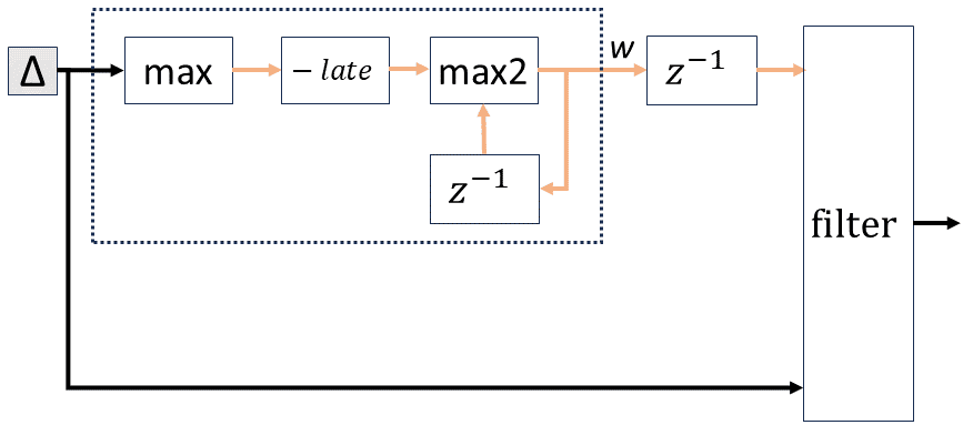
The following diagram shows how the LATENESS information is synthesized into a DBSP circuit. (We haven't really talked about DBSP circuits in this blog, think of such circuits as dataflow graphs, or query plans; each box is an operator, and each arrow is data).

One such circuit is synthesized right after each table or view that has LATENESS annotations. The table is the leftmost block, labeled Δ. This block receives at every step from an input adapter the latest changes to the table, in the form of a Z-set.

The dotted line rectangle is the circuit that computes the waterline of the data. The waterline is on the red arrow labeled w. In the picture the black arrows carry changes in the form of Z-sets, while the red arrows carry single values.

The waterline is computed by three blocks:

• the first max block receives as input a Z-set (a collection containing all the rows inserted or deleted). The block iterates over all the rows and computes the maximum of the timestamp column. The input is a collection (black arrow), while the output is a single value.
  Let's assume the input has two records with timestamps: 2024-01-01 10:00:00 and 2024-01-01 10:00:01. The result of the max block is 2024-01-01 10:00:01.
• the second block subtracts the declared lateness value from the
  resulting max. In our example the output would be 2024-01-01
09:00:01
• the max2 block has two inputs: the output of the subtraction, and its own output, delayed by one step (that's what the z-1 operator does: it emits its input one step later). When the circuit starts, the first output of the delay is the minimum timestamp possible, in this case 0001-00-00 00:00:00. So the output of the max block after the first step is 2024-01-01 09:00:01.

This is the value of the waterline computed after the first input has
been processed. (If there is no data in the first input then the waterline value
is minimum legal timestamp.)

Notice that the waterline value w will increase (or stay the same) at each step, because it is the max of its prior value and the next one, computed by the max2 block.

Filtering out late data

The waterline computed is used to filter data. The filter block shown is similar to a SQL WHERE filter, but it has a black and a red input; it actually compares the timestamp of every input record from the black arrow with the waterline from the red input. Records that are below the waterline are discarded. This ensures that only records that obey the LATENESS promise are sent to the rest of the pipeline for processing. Even if the input produces late data, the rest of the pipeline will never see it. This invariant is used by our optimizer to GC data from the rest of the circuit.

Notice that the waterline is fed through a delay to the filter block. This means that a waterline takes effect in the next step of a circuit. The waterline computed from the first input change is only used to filter data from the second change.

Computing the waterline does not involve any clocks: all the timestamps are extracted from the events themselves.

One can thus think of a Feldera SQL program as having two parts:

• the LATENESS annotations, which clean-up late data
• 100% standard SQL queries that produce the expected results: at each step, each output view reflects the data received in all input tables

If data never arrives late, then any query will produce exactly the same results, with or without LATENESS annotations on the sources. But the query with LATENESS can also GC data, while the one without cannot.

It is important to understand that LATENESS does not delay the processing of the data or production of results in any way. If the IRS runs a query on January 1, it will get the correct result with respect to all the data that has arrived by Jan 1. If the IRS runs a query on April 15, it will get the correct result with respect to all the data that has arrived by April 15. The difference made by lateness is the following:

When using LATENESS, after April 15 the IRS knows that the results of any query analyzing the data of the prior year will never change, even if more records for the prior year arrive late.

(This makes the system vulnerable to a denial-of-service attack from a defective event source: by sending an event with a timestamp very far in the future, the source can cause all other input records to be discarded. Other mechanisms can be used to protect against this scenario, but they all require the system to have access to a real-time clock that can be trusted.)

In a future blog post we will also show how Feldera computes waterlines not just for the input collection, but also for collections that are produced by SQL operators from the input collections. The waterline allows the Feldera runtime to GC data. Because some input tables in streaming programs grow continuously, as do some intermediate results, the waterline is crucial to keep the computation running for long stretches of time without running out of memory and without producing incorrect results.

Conclusions

Designing a new programming language is fraught with peril. Reusing an existing language, especially a well-known language, is always preferable. Streaming systems started by designing custom languages, but gradually adopted SQL. An important goal in adapting SQL for stream processing is to minimally modify SQL such that standard SQL programs have the exact same behavior as in normal databases. In this post we have presented a type annotation called LATENESS which can be used to filter out of order data, and we have given a very precise definition of its behavior. The beauty of LATENESS is the ease of use: you annotate a data source, and then you can forget about it, and all queries will behave exactly like standard SQL queries, except that they will not process late data.