Taking the short path to streaming on the GPU with DBSP

Community Spotlight: This post was contributed by a Feldera community member.

The power behind the simplicity of Feldera’s underlying theory

In this blog there has been much discussion about Feldera’s performance. Many improvements stem from pushing the envelope on the Rust implementation of DBSP, the powerful theory that assures you that not only is Feldera a sound stream processing engine, but an efficient one as well.

In a previous blog post, Feldera was shown to be on average 2.2 times faster than Flink while consuming 4 times less memory.

How is it possible that Feldera is this fast already, having had orders-of-magnitude-fewer hours of development having been put into it?

The key - I believe - lies in DBSP. It is simple, general, and provides a practical mental model to the cost, both in time and in data, of computations.

In this post we will put this to practice by leveraging a Python implementation of DBSP to implement incremental relational operators that show noticeable speed improvements.

We will start with an inefficient join over sets and go all the way to incremental streaming joins on the GPU (in one post).

The goal is so that by the end of this reading not only will you be able to grasp how “incremental” stream processing differs from batch and not-incremental streaming, but also that the expected performance improvements are not tied to hardware nor are they specific to the Rust implementation.

Here you can find a jupyter notebook with all the plots and code.

Let there be joins

from typing import List, Tuple, Set

def regular_join[K, V1, V2](left: Set[Tuple[K, V1]], right: Set[Tuple[K, V2]]) -> List[Tuple[K, V1, V2]]:
  output: List[Tuple[K, V1, V2]] = []
  for left_key, left_value in left:
    for right_key, right_value in right:
      if left_key == right_key:
        output.append((left_key, left_value, right_value))

return output

employees = {(0, "kristjan"), (1, "mark"), (2, "mike")}
salaries = {(2, "40000"), (0, "38750"), (1, "50000")}

employees_salaries = regular_join(employees, salaries)
print(f"Regular join: {employees_salaries}")
# Regular join: [(1, 'mark', '50000'), (2, 'mike', '40000'), (0, 'kristjan', '38750')]

The function regular_join is a straightforward relational inner join implementation. Given two relations, by looping over them with some key, the output are all rows that match.

from pydbsp.zset import ZSet
from pydbsp.zset.functions.bilinear import join

employees_zset = ZSet({k: 1 for k in employees})
salaries_zset = ZSet({k: 1 for k in salaries})
employees_salaries_zset = join(
  employees_zset,
  salaries_zset,
  lambda left, right: left[0] == right[0],
  lambda left, right: (left[0], left[1], right[1]),
)
print(f"ZSet join: {employees_salaries_zset}")
# ZSet join: {(1, 'mark', '50000'): 1, (2, 'mike', '40000'): 1, (0, 'kristjan', '38750'): 1}

Let us now go from joining relations to doing so over their more general siblings, ZSet relations.

ZSets form a scary-named mathematical construct, the Abelian group. An abelian group is nothing but a set with associated + and - operations. If you would prefer a more thorough and precise introduction, check this blog post out.

class ZSet[T]:
    inner: Dict[T, int]

    def __init__(self, values: Dict[T, int]) -> None:
        self.inner = values

    def items(self) -> Iterable[Tuple[T, int]]:
        """Returns an iterable of (element, weight) pairs."""
        return self.inner.items()

    def __contains__(self, item: T) -> bool:
        """An item is in the Z-set if it has non-zero weight."""
        return self.inner.__contains__(item)

    def __getitem__(self, item: T) -> int:
        """Returns the weight of an item (0 if not present)."""
        if item not in self:
            return 0

        return self.inner[item]

    def is_identity(self) -> bool:
        return len(self.inner) == 0

The only difference is that while relations could be interpreted as sets of items that each share the same “columns”, ZSet relations take this a step further by associating each item with a weight.

When one adds two of these, the result is the union of both sets with the weights of identical elements summed.Negation is as straightforward as it sounds. One just flips the sign on each element's weight.

class ZSetAddition[T]:
    def add(self, a: ZSet[T], b: ZSet[T]) -> ZSet[T]:
        result = a.inner | b.inner

        for k, v in b.inner.items():
            if k in a.inner:
                new_weight = a.inner[k] + v
                if new_weight == 0:
                    del result[k]
                else:
                    result[k] = new_weight

        return ZSet(result)

    def neg(self, a: ZSet[T]) -> ZSet[T]:
        return ZSet({k: v * -1 for k, v in a.inner.items()})

    def identity(self) -> ZSet[T]:
        return ZSet({})

Notice how it is possible to model regular sets, bags and set updates with them.

A set is a ZSet where each weight is exactly 1, a bag is where it can be more than 1, and a diff is one where it is either 1 or -1.Diffs are the most important for us, as they are the key to make things “incremental” and play quite nicely with the concept of function linearity.

Efficiently incrementalizing linear functions

Certain kinds of functions, the ones that are linear, can be efficiently and predictably “incrementalized”. If you would like a more thorough and unambiguous take on what “incremental” means, see here.

Many useful functions are `linear`. For instance, regular_join is. A function is linear, or bilinear if it has two arguments, if it distributes over addition. In our case, ZSet addition.

Better put, for some function f, it is linear over the ZSet addition group if for each a, b that are ZSets, it holds: f(a + b) = f(a) + f(b).

This might be a tad abstract, but let's garner some intuition by first looking at it from the relational selection perspective, and then how when applied to joins it gives a blueprint to make it “incremental”.

The “select” (σ) operation on some relation filters it according to some predicate p. Taking E as the ZSet of salaries, and ΔE as some diff of salaries, it is trivial to see that σ(E + ΔE)p = σ(E)p + σ(ΔE)p, hence It is linear.

Linear functions are already incremental when lifted, as the time it takes to update the computation is proportional to the size of the diff.

Now onto a more involved example where linearity, in this case bilinearity, does not immediately imply being incremental, but implies the existence of an incremental form.

The join of the running example has been, taking S as the salary ZSet: E ⨝ S

If we call ΔS as the set of diffs to S, the "batch" way of evaluating this query under an update would be: (E + ΔE) ⨝ (S + ΔS)

Since it distributes over addition, we could also evaluate it incrementally: (ΔE) ⨝ (ΔS) + (E) ⨝ (ΔS) + (ΔE) ⨝ (S).

When done that way, three joins happen instead of one. Notice however how at least one side of each join is a diff. This makes it much more efficient, since we effectively shift the lower bound from "all data" to "the diff".

And that’s pretty much it. Putting it succinctly, computations are “incremental” if the worst case is bounded by the size of the diff.

Interestingly, this also implies that not all stream processing is incremental.

Incremental vs non-incremental streaming joins

from pydbsp.zset import ZSetAddition
from pydbsp.stream import Stream, StreamHandle
from pydbsp.stream.operators.linear import Integrate
from pydbsp.zset.operators.bilinear import LiftedJoin

group = ZSetAddition()
employees_stream = Stream(group)
employees_stream_handle = StreamHandle(lambda: employees_stream)
employees_stream.send(employees_zset)

salaries_stream = Stream(group)
salaries_stream_handle = StreamHandle(lambda: salaries_stream)
salaries_stream.send(salaries_zset)

join_cmp = lambda left, right: left[0] == right[0]
join_projection = lambda left, right: (left[0], left[1], right[1])

integrated_employees = Integrate(employees_stream_handle)
integrated_salaries = Integrate(salaries_stream_handle)
stream_join = LiftedJoin(
    integrated_employees.output_handle(),
    integrated_salaries.output_handle(),
    join_cmp,
    join_projection,
)
integrated_employees.step()
integrated_salaries.step()
stream_join.step()
print(f"ZSet stream join: {stream_join.output().latest()}")
# ZSet stream join: {(1, 'mark', '50000'): 1, (2, 'mike', '40000'): 1, (0, 'kristjan', '38750'): 1}

Now, streams. Let’s keep it simple and consider them to be infinite lists.

We say that to lift some function is to apply it element-wise to some stream as data “arrives”.

LiftedJoin in the example is join applied element-wise to two ZSet streams. The result of the stream join is then predictably the same as the regular ZSet join.

Integrate is an operator, a function whose input and output are streams, that at each time step contains the cumulative sum of all values so far. It is very important.

When a stream of updates is integrated, at each timestep we have the “full” data. This is a potentially expensive operation.

A non-incremental “streaming” join then is one that computes (E + ΔE) ⨝ (S + ΔS) at each timestep, where ΔE and ΔS are the batches that arrived at that timestamp.

from pydbsp.stream.operators.bilinear import Incrementalize2

incremental_stream_join = Incrementalize2(
    employees_stream_handle,
    salaries_stream_handle,
    lambda left, right: join(left, right, join_cmp, join_projection),
    group,
)
incremental_stream_join.step()
print(f"Incremental ZSet stream join: {incremental_stream_join.output().latest()}")
# Incremental ZSet stream join: {(0, 'kristjan', '38750'): 1, (1, 'mark', '50000'): 1, (2, 'mike', '40000'): 1}

Due to the bi-linearity of join, we can immediately make it "incremental" - as seen in the previous section - by using the Incrementalize2 operator. One of its arguments is the function to “incrementalize”, which in our case is the ZSet join.

It then automatically assembles an operator that, at each timestamp computes: (ΔE) ⨝ (ΔS) + (E) ⨝ (ΔS) + (ΔE) ⨝ (S)

employees_stream.send(ZSet({(2, "mike"): -1}))
incremental_stream_join.step()
print(f"Incremental ZSet stream join update: {incremental_stream_join.output().latest()}")
# Incremental ZSet stream join update: {(2, 'mike', '40000'): -1}

Modern streaming systems often handle deletion poorly, and often they just don't. ZSets however give us this for free.

If we send in a ZSet with some elements that have negative weight, they will cancel the corresponding elements with positive weights. This will “propagate” through any downstream operator.

In this example, by retracting mike the result of the join will also get retracted.

So far we went from batch all the way to incremental stream processing with very few lines of code, relying entirely on theory.

Indexes

from pydbsp.indexed_zset.functions.bilinear import join_with_index
from pydbsp.indexed_zset.operators.linear import LiftedIndex

indexer = lambda x: x[0]
index_employees = LiftedIndex(employees_stream_handle, indexer)
index_salaries = LiftedIndex(salaries_stream_handle, indexer)
incremental_sort_merge_join = Incrementalize2(index_employees.output_handle(), index_salaries.output_handle(), lambda l, r: join_with_index(l, r, join_projection), group)
index_employees.step()
index_salaries.step()
incremental_sort_merge_join.step()
print(f"Incremental indexed ZSet stream join: {incremental_sort_merge_join.output().latest()}")
# Incremental indexed ZSet stream join: {(0, 'kristjan', '38750'): 1, (1, 'mark', '50000'): 1, (2, 'mike', '40000'): 1}

There are multiple ways to implement joins. The three most common kinds are:

1. Hash

2. Nested loop

3. Sort-merge

Adding b-tree indexes to a database table makes 3., often the most efficient, possible.

Our regular_join is a nested loop join. Are we also able to somehow add "indexes" to our

streams and take advantage of sort-merge joins?

Yes! Index building is linear. The LiftedIndex operator incrementally indexes both employees and salaries by their first column.

Indexing streams is a must. Check the blog post on Indexed ZSets to understand how they are different from regular ZSets, and what kind of operations they enable.

Benchmarks

from random import randrange

names = ("kristjan", "mark", "mike")
max_pay = 100000
fake_data = [((i, names[randrange(len(names))] + str(i)), (i, randrange(max_pay))) for i in range(3, 10003)]
batch_size = 500
fake_data_batches = [fake_data[i : i + batch_size] for i in range(0, len(fake_data), batch_size)]

for batch in fake_data_batches:
    employees_stream.send(ZSet({employee: 1 for employee, _ in batch}))
    salaries_stream.send(ZSet({salary: 1 for _, salary in batch}))

steps_to_take = len(fake_data_batches)

By now we have implemented many variations of a streaming join:

1. Batch

2. Incremental

3. Incremental with indexing

To compare all of these we will run a simple benchmark using not a lot of data. As the snippet above shows, there will be 20 batches with each containing 500 employees and salaries.

And for the cherry on top, let's add one more variant, this time using Pandas as the back-end. This will also show just how easily it is to implement a ZSet on top of other data structures.

from tqdm.notebook import tqdm
from time import time

time_start = time()
measurements = []
for _ in tqdm(range(steps_to_take)):
    local_time = time()
    integrated_employees.step()
    integrated_salaries.step()
    stream_join.step()
    measurements.append(time() - local_time)
print(f"Time taken - on demand: {time() - time_start}s")
# Time taken - on demand: 20.124440670013428s

Computing all 200 batches with a regular stream join took a whopping...20 seconds.

That is very slow. We have an excuse however. The goal of the baseline ZSet implementation is to be simple to understand and to debug.

import pandas as pd

time_start = time()
pandas_measurements = []
employees_union_df = pd.DataFrame(columns=['id', 'name'])
salaries_union_df = pd.DataFrame(columns=['id', 'salary'])

for step in tqdm(range(steps_to_take)):
    local_time = time()
    employees_batch_df = pd.DataFrame([ employee for employee, _ in fake_data_batches[step] ], columns=['id', 'name'])
    employees_union_df = pd.concat([employees_union_df, employees_batch_df], ignore_index=True)

    salaries_batch_df = pd.DataFrame([ salary for _, salary in fake_data_batches[step] ], columns=['id', 'salary'])
    salaries_union_df = pd.concat([salaries_union_df, salaries_batch_df], ignore_index=True)
    
    employees_x_salaries = pd.merge(employees_union_df, salaries_union_df, on=['id'], how='inner')
    pandas_measurements.append(time() - local_time)

print(f"Time taken - on demand with pandas: {time() - time_start}s")
# Time taken - on demand with pandas: 0.032193899154663086s

Pandas blew it out of the water being 666 times faster.

How fast can we make it then by:

Making it incremental?
Adding indexes?

time_start = time()
incremental_measurements = []
for _ in tqdm(range(steps_to_take)):
    local_time = time()
    incremental_stream_join.step()
    incremental_measurements.append(time() - local_time)
print(f"Time taken - incremental: {time() - time_start}s")
# Time taken - incremental: 2.9529590606689453s

With the incremental variant of the stream join we get a 6.66 times improvement. It nonetheless still is 100 times slower than recomputing from scratch at each new timestamp with pandas.

time_start = time()
incremental_with_index_measurements = []
for _ in tqdm(range(steps_to_take)):
    local_time = time()
    index_employees.step()
    index_salaries.step()
    incremental_sort_merge_join.step()
    incremental_with_index_measurements.append(time() - local_time)
print(f"Time taken - incremental with index: {time() - time_start}s")
# Time taken - incremental with index: 0.16031384468078613s

This graph shows the time taken to process each timestamp. The x axis is the timestamp and y is the latency.

Each line contains the measurements from each of the previous benchmarks. The batch series stands for the non-incremental streaming join, batch`pd for non-incremental streaming with pandas, inc for incremental, and inc_idx for incremental with indexing.

Indexing makes a big difference. With almost no change in code it is more than 100 times faster than the original batch solution.

Now we are only down to being 5.33 times slower than pandas using pure python and the power of DBSP.

batch_size = 100000

lots_of_fake_data = [((i, names[randrange(len(names))] + str(i)), (i, randrange(max_pay))) for i in range(10000000)]
lots_of_fake_data_batches = [lots_of_fake_data[i : i + batch_size] for i in range(0, len(lots_of_fake_data), batch_size)]

new_pandas_measurements = []
employees_union_df = pd.DataFrame(columns=['id', 'name'])
salaries_union_df = pd.DataFrame(columns=['id', 'salary'])
new_steps_to_take = len(lots_of_fake_data_batches)
results_pandas = [] 

time_start = time()
for step in tqdm(range(new_steps_to_take)):
    local_time = time()
    employees_batch_df = pd.DataFrame([ employee for employee, _ in lots_of_fake_data_batches[step] ], columns=['id', 'name'])
    employees_union_df = pd.concat([employees_union_df, employees_batch_df], ignore_index=True)

    salaries_batch_df = pd.DataFrame([ salary for _, salary in lots_of_fake_data_batches[step] ], columns=['id', 'salary'])
    salaries_union_df = pd.concat([salaries_union_df, salaries_batch_df], ignore_index=True)
    
    employees_x_salaries = pd.merge(employees_union_df, salaries_union_df, on='id', how='inner')
    results_pandas.append(employees_x_salaries)
    new_pandas_measurements.append(time() - local_time)

print(f"Time taken - on demand with pandas: {time() - time_start}s")
# Time taken - on demand with pandas: 97.98046684265137s

Let's scale up the data size. At what point does pandas start to struggle? If we shift the batch up to 100000 new employees and salaries, and push 100 of these, pandas

takes around 97 seconds to churn through.

Could we leverage DBSP to speed pandas up?

from pydbsp.core import AbelianGroupOperation

class ImmutableDataframeZSet:
    inner: List[pd.DataFrame]
    
    def __init__(self, df: pd.DataFrame) -> None:
        if 'weight' not in df.columns:
            raise ValueError("DataFrame must have a 'weight' column")
        self.inner: List[pd.DataFrame] = [df[df['weight'] != 0]]

    def __repr__(self) -> str:
        return self.inner.__repr__()

    def __eq__(self, other: object) -> bool:
        if not isinstance(other, ImmutableDataframeZSet):
            return False
        if len(self.inner) != len(other.inner):
            return False
        return all(df1 is df2 for df1, df2 in zip(self.inner, other.inner))

This class is a mostly compliant “lazy” pandas-backed ZSet with a very loose pointer-based equality mechanism. Equality here only works if both ZSets hold pointers of the same underlying dataframes.

class ImmutableDataframeZSetAddition(AbelianGroupOperation[ImmutableDataframeZSet]):
    def add(self, a: ImmutableDataframeZSet, b: ImmutableDataframeZSet) -> ImmutableDataframeZSet:
        if not a.inner:
            return b

        if not b.inner:
            return b
            
        result = ImmutableDataframeZSet(pd.DataFrame(columns=a.inner[0].columns))
        result.inner = a.inner + b.inner
        return result

    def neg(self, a: ImmutableDataframeZSet) -> ImmutableDataframeZSet:
        result = ImmutableDataframeZSet(pd.DataFrame(columns=a.inner[0].columns))
        result.inner = [df.assign(weight=lambda x: -x.weight) for df in a.inner]
        return result

    def identity(self) -> ImmutableDataframeZSet:
        return ImmutableDataframeZSet(pd.DataFrame(columns=['weight']))

Defining abelian addition over it is straightforward. Adding two lists is the same as concatenating them, negating is iterating over each dataframe and negating the weight column, and identity for addition is a ZSet with a single dataframe containing no rows.

employees_dfs_stream = Stream(immutable_df_abelian_group)
employees_dfs_stream_handle = StreamHandle(lambda: employees_dfs_stream)

salaries_dfs_stream = Stream(immutable_df_abelian_group)
salaries_dfs_stream_handle = StreamHandle(lambda: salaries_dfs_stream)

incremental_pandas_join = Incrementalize2(employees_dfs_stream_handle, salaries_dfs_stream_handle, lambda l, r: immutable_dataframe_zset_join(l, r, ['id']), immutable_df_abelian_group)
incremental_pandas_measurements = []
time_start = time()
for step in tqdm(range(new_steps_to_take)):
    local_time = time()
    employees_batch_df = pd.DataFrame([ employee + (1,) for employee, _ in lots_of_fake_data_batches[step] ], columns=['id', 'name', 'weight'])
    employees_dfs_stream.send(ImmutableDataframeZSet(employees_batch_df))
    
    salaries_batch_df = pd.DataFrame([ salary + (1,) for _, salary in lots_of_fake_data_batches[step] ], columns=['id', 'salary', 'weight'])
    salaries_dfs_stream.send(ImmutableDataframeZSet(salaries_batch_df))
        
    incremental_pandas_join.step()
    incremental_pandas_measurements.append(time() - local_time)
print(f"Time taken - incremental: {time() - time_start}s")
# Time taken - incremental: 20.01264476776123s

A join is implemented by joining all pairs and adding the results. And voila! Doing things “incrementally” is more than 4 times faster.

But what about the title? The choice of Pandas was not random. We can make this implementation use a GPU by changing a single line of code.

import cudf as cu

class ImmutableGPUDataframeZSet:
    def __init__(self, df: cu.DataFrame) -> None:
        if 'weight' not in df.columns:
            raise ValueError("DataFrame must have a 'weight' column")
        self.inner: List[cu.DataFrame] = [df[df['weight'] != 0]]

    def __repr__(self) -> str:
        return self.inner.__repr__()

    def __eq__(self, other: object) -> bool:
        if not isinstance(other, ImmutableGPUDataframeZSet):
            return False
        if len(self.inner) != len(other.inner):
            return False
        return all(df1 is df2 for df1, df2 in zip(self.inner, other.inner))

We just need to change the import from pd to cu, and then our whole streaming system can now run on a GPU.

How will our humble mobile RTX 3070 fare?

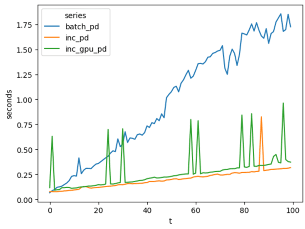
This graph has the same shape and intent as the previous one. The x axis is each timestamp, and the y is the latency in seconds.

Each series contains the latency measured for each timestamp in the large benchmark. batch_pd represents non-incremental pandas, inc_pd uses the pandas-backed ZSets and incremental operators, and inc_gpu_pd does so using the GPU.

The total runtime for inc_gpu_pd was 27 seconds, 7 seconds more than inc_pd. While using a GPU was slower than not, it was still remarkable given that this is an old mobile GPU. Perhaps with a faster one there could be a speedup.

Conclusion

In this blog post we described some of the most practical aspects of the theory that powers Feldera, DBSP, and saw how it allows for clearly differentiating between incremental and not-so-incremental streaming joins.

Furthermore, as it is quite general, we were able to run the same code both in the GPU and CPU, which brings us back to the title. Could Feldera one day leverage GPU acceleration? Yes, it could.

Taking the short path to streaming on the GPU with DBSP

The power behind the simplicity of Feldera’s underlying theory

Let there be joins

Efficiently incrementalizing linear functions

Incremental vs non-incremental streaming joins

Indexes

Benchmarks

Conclusion

Other articles you may like

Incremental Update 6 at Feldera

Database computations on Z-sets

Incremental Update 5 at Feldera