Real-time feature engineering with Feldera. Part 2.

In the previous blog post we introduced the real-time feature engineering problem. That is, how does one transform continuously arriving raw data into feature vectors in real-time to supply an ML model with up-to-date features. We discussed how current streaming analytics tools are restrictive, unreliable, and hard to use.

We then hinted at the shape of an ideal solution: one that allows users to rapidly iterate on complex feature queries during feature exploration, and then run those exact same queries at scale in production for both model training and real-time inference.

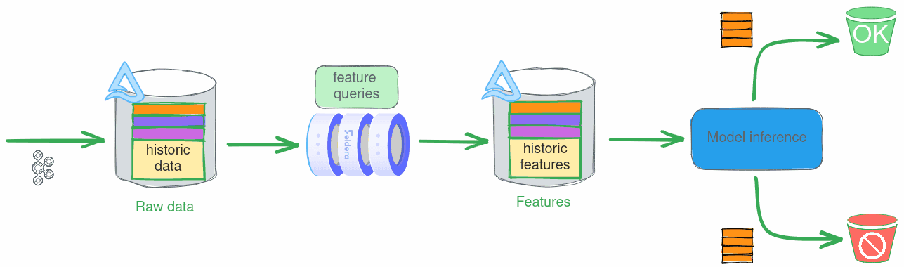
In this blog post we show how Feldera implements this vision through a practical example, credit card fraud detection:

• We write an SQL query that defines several interesting features, based on
  data enrichment and rolling aggregates.
• We use this query to compute feature vectors with Feldera and train an ML model on a historical data set stored in a Delta Lake.
• We use the same query to compute feature vectors over a real-time stream of credit card transaction data. By simply connecting new data sources and sinks, the SQL query we used for training the model on batch inputs works seamlessly on streaming data.
• We do all this from the comfort of a Python notebook environment familiar to
  most ML engineers.

Credit card fraud detection

Credit card fraud detection is a classic application of real-time feature engineering. Here, data comes in a stream of transactions, each with attributes like card number, purchase time, vendor, and amount. Additionally, the fraud detector has access to a slowly changing table with demographics information about cardholders, such as age and address.

We use a publicly available Synthetic Credit Card Transaction Generator to generate transaction data for 1000 user profiles.

We define several features over these inputs:

• Data enrichment:
  • We add demographic attributes, such as zip code, to each transaction
• Rolling aggregates:
  • average spending per transaction in the past day, week, and month
  • average spending per transaction over a 3-month timeframe on the same day of the week
  • number of transactions made with this credit card in the last 24 hours
• Other:
  • is_weekend - transaction took place on a weekend
  • is_night - transaction took place before 6am
  • d - day of week

These features are representative of real-world feature engineering practices, which we will cover in more detail in future posts.

To ground the parameters of the problem further, we assume that both raw inputs and computed feature vectors are stored in a Delta Lake, which is a platform of choice for many data and ML teams today.

Training

Finding an optimal set of features to train a good ML model is an iterative process. At every step, the data scientist trains and tests a model using currently selected feature queries on an array of labeled historical data. The results of each experiment drive the next refinement of feature queries. In this scenario, feature vectors are computed in batch mode over a slice of historical data, e.g., data collected over a two-week timeframe.

The following Python function creates a SQL program, consisting of two tables with raw input data (`TRANSACTION` and `DEMOGRAPHICS`) and the `FEATURE` view, which defines several features over these tables. The function can be used to instantiate the pipeline with different sources and sinks, by invoking it with different connector configurations.

def build_program(transactions_connectors: str, demographics_connectors: str, features_connectors: str) -> str:
  return f"""-- Credit card transactions
    CREATE TABLE TRANSACTION(
      trans_date_trans_time TIMESTAMP,
      cc_num BIGINT,
      merchant STRING,
      category STRING,
      amt DOUBLE,
      trans_num STRING,
      unix_time BIGINT,
      merch_lat DOUBLE,
      merch_long DOUBLE,
      is_fraud BIGINT
    ) WITH ('connectors' = '{transactions_connectors}');
    
    -- Demographics data.
    CREATE TABLE DEMOGRAPHICS(
      cc_num BIGINT,
      first STRING,
      last STRING,
      gender STRING,
      street STRING,
      city STRING,
      state STRING,
      zip BIGINT,
      lat DOUBLE,
      long DOUBLE,
      city_pop BIGINT,
      job STRING,
      dob DATE
    ) WITH ('connectors' = '{demographics_connectors}');
    
    -- Feature query written in the Feldera SQL dialect.
    CREATE VIEW FEATURE
    WITH ('connectors' = '{features_connectors}')
    AS
    SELECT
      t.cc_num,
      dayofweek(trans_date_trans_time) as d,
      CASE
      WHEN dayofweek(trans_date_trans_time) IN(6, 7) THEN true
      ELSE false
      END AS is_weekend,
      hour(trans_date_trans_time) as hour_of_day,
      CASE
      WHEN hour(trans_date_trans_time) <= 6 THEN true
      ELSE false
      END AS is_night,
      -- Average spending per day, per week, and per month.
      AVG(amt) OVER window_1_day AS avg_spend_pd,
      AVG(amt) OVER window_7_day AS avg_spend_pw,
      AVG(amt) OVER window_30_day AS avg_spend_pm,
      -- Average spending over the last three months for the same day of the week.
      COALESCE(
      AVG(amt) OVER (
      PARTITION BY t.cc_num, EXTRACT(DAY FROM trans_date_trans_time)
      ORDER BY unix_time
      RANGE BETWEEN 7776000 PRECEDING and CURRENT ROW
      ), 0) AS avg_spend_p3m_over_d,
      -- Number of transactions in the last 24 hours.
      COUNT(*) OVER window_1_day AS trans_freq_24,
      amt, unix_time, zip, city_pop, is_fraud
    FROM transaction as t
    JOIN demographics as d
      ON t.cc_num = d.cc_num
    WINDOW
      window_1_day AS (PARTITION BY t.cc_num ORDER BY unix_time RANGE BETWEEN 86400 PRECEDING AND CURRENT ROW),
      window_7_day AS (PARTITION BY t.cc_num ORDER BY unix_time RANGE BETWEEN 604800 PRECEDING AND CURRENT ROW),
      window_30_day AS (PARTITION BY t.cc_num ORDER BY unix_time RANGE BETWEEN 2592000 PRECEDING AND CURRENT ROW);
"""

Next, we instantiate the pipeline to read training data for transaction and demographics tables from two Delta tables stored in a public S3 bucket, and to write the contents of the `FEATURE` view to another Delta table in a private S3 bucket. We use the Feldera Python SDK to connect to a Feldera service (here we use the Feldera online sandbox) and run the pipeline.

from feldera import FelderaClient, PipelineBuilder

# S3 access credentials.
S3_CONFIG = {
  "aws_access_key_id": AWS_ACCESS_KEY_ID,
  "aws_secret_access_key": AWS_SECRET_ACCESS_KEY,
  "aws_region": "us-east-1"
}

# Load DEMOGRAPHICS data from a Delta table stored in an S3 bucket.
demographics_connectors = [{
  "transport": {
    "name": "delta_table_input",
    "config": {
      "uri": "s3://feldera-fraud-detection-data/demographics_train",
      "mode": "snapshot",
      "aws_skip_signature": "true"
    }
  }
}]

# Load credit card TRANSACTION data.
transactions_connectors = [{
  "transport": {
    "name": "delta_table_input",
    "config": {
      "uri": "s3://feldera-fraud-detection-data/transaction_train",
      "mode": "snapshot",
      "aws_skip_signature": "true",
      "timestamp_column": "unix_time"
    }
  }
}]

features_connectors = [{
  "transport": {
    "name": "delta_table_output",
    "config": {
      "uri": f"s3://feldera-fraud-detection-demo/feature_train",
      "mode": "truncate"
      } | S3_CONFIG
    }
}]

# Connect to Feldera.
# Use the 'Settings' menu at try.feldera.com to generate an API key.
client = FelderaClient("https://try.feldera.com", api_key = FELDERA_API_KEY)

sql = build_program(json.dumps(transactions_connectors), json.dumps(demographics_connectors), json.dumps(features_connectors))

pipeline = PipelineBuilder(client, name="fraud_detection_training", sql=sql).create_or_replace()

# Process full snapshot of the input tables and compute a dataset
# with feature vectors for use in model training and testing.
pipeline.start()
pipeline.wait_for_completion(shutdown=True)

Computed features are now stored in `s3://feldera-fraud-detection-demo/feature_training` and can be used to train and test the model:

Import computed features to the Databricks environment.

create table if not exists feature_train location 's3://feldera-fraud-detection-demo/feature_train';

Data preparation

from pyspark.ml.feature import VectorAssembler

def feature_vectorization(dataframe):
  assembler = VectorAssembler(
    inputCols=["cc_num", "d", "hour_of_day", "is_weekend", "is_night", "avg_spend_pd", "avg_spend_pw", "avg_spend_pm", "avg_spend_p3m_over_d", "trans_freq_24", "amt", "unix_time", "city_pop"],
    outputCol='feature_vector',
    handleInvalid='skip'
  )
  data_transformed = assembler.transform(dataframe)
  return data_transformed

df_train_test = spark.sql("SELECT * FROM feature_train")
transformed_df = feature_vectorization(df_train_test)

# Split dataset into train and test tables.
train, test = transformed_df.randomSplit([0.7, 0.3], seed = 42)

Training and testing

from pyspark.ml import Pipeline
from pyspark.ml.classification import DecisionTreeClassifier
from pyspark.ml.classification import DecisionTreeClassificationModel

# Model specification
dt = DecisionTreeClassifier(
  featuresCol = "feature_vector",
  labelCol = "is_fraud"
)
pipeline = Pipeline(stages = [dt])

# Training
model = pipeline.fit(train)

# Testing
predictions = model.transform(test)
prediction = predictions.select("prediction", "is_fraud")

from pyspark.ml.evaluation import BinaryClassificationEvaluator, MulticlassClassificationEvaluator

def evaluate_model(prediction_df, prediction_name):

binary_evaluator = BinaryClassificationEvaluator(
rawPredictionCol="prediction", labelCol="is_fraud", metricName="areaUnderPR")
areaUnderPR = binary_evaluator.evaluate(prediction_df)

multi_evaluator = MulticlassClassificationEvaluator(labelCol="is_fraud", predictionCol="prediction")

# Specifying "is_fraud" as positive label we want to evaluate
precision = multi_evaluator.setMetricName("precisionByLabel").evaluate(prediction_df, {multi_evaluator.metricLabel: 1.0})
recall = multi_evaluator.setMetricName("recallByLabel").evaluate(prediction_df, {multi_evaluator.metricLabel: 1.0})
f1_score = multi_evaluator.setMetricName("f1").evaluate(prediction_df)

if prediction_name == "batch_prediction":
  print(f"Area Under PR for current batch: {areaUnderPR * 100:.2f}%")
  print(f"Precision for current batch: {precision * 100:.2f}%")
  print(f"Recall for current batch: {recall * 100:.2f}%")
  print(f"F1 Score for current batch: {f1_score * 100:.2f}%")
else:
  print(f"Area Under PR: {areaUnderPR * 100:.2f}%")
  print(f"Precision: {precision * 100:.2f}%")
  print(f"Recall: {recall * 100:.2f}%")
  print(f"F1 Score: {f1_score * 100:.2f}%")

evaluate_model(prediction, "prediction")

Computed model metrics

If you have done feature engineering before, you will find that this workflow is similar to model training using Spark or Pandas. Here comes the pleasant surprise: **the above code also works in streaming mode, all you have to do is connect new data sources and sinks!**

Real-time inference

During real-time feature computation, raw data arrives from a streaming
source like Kafka. Feldera can ingest data directly from such sources, but in
this case we will assume that Kafka is connected to a Delta table, and configure
Feldera to ingest the data by following the transaction log of the table.

There are several advantages to using this setup in production, but it is also great
for demos, as it allows us to stream data from a pre-filled table without having to
manage a Kafka queue.

The code below is almost identical to our training setup, except that this time
we use synthetic live data instead of training data. We configure the input
connector for the `TRANSACTION` table to ingest transaction data in the
snapshot-and-follow mode. In this mode, the connector reads the initial
snapshot of the table before following the stream of changes in its transaction
log.

# Load DEMOGRAPHICS data from a Delta table.
demographics_connectors = [{
  "transport": {
    "name": "delta_table_input",
    "config": {
      "uri": "s3://feldera-fraud-detection-data/demographics_infer",
      "mode": "snapshot",
      "aws_skip_signature": "true"
    }
  }
}]

# Read TRANSACTION data from a Delta table.
# Configure the Delta Lake connector to read the initial snapshot of
# the table before following the stream of changes in its transaction log.
transactions_connectors = [{
  "transport": {
    "name": "delta_table_input",
    "config": {
      "uri": "s3://feldera-fraud-detection-data/transaction_infer",
      "mode": "snapshot_and_follow",
      "version": 10,
      "timestamp_column": "unix_time",
      "aws_skip_signature": "true"
    }
  }
}]

# Store computed feature vectors in another delta table.
features_connectors = [{
  "transport": {
    "name": "delta_table_output",
    "config": {
      "uri": f"{args.deltalake_uri}/feature_infer",
      "mode": "truncate"
      } | S3_CONFIG,
    }
}]

sql = build_program(json.dumps(transactions_connectors), json.dumps(demographics_connectors), json.dumps(features_connectors))
pipeline = PipelineBuilder(client, name="fraud_detection_inference", sql=sql).create_or_replace()

# Start the pipeline to continuously process the input stream of credit card
# transactions and output newly computed feature vectors to a Delta table.

pipeline.start()

Feldera now runs in the background, continuously ingesting new credit card
transaction records and computing new feature vectors in real-time. We can monitor its progress in the WebConsole.

We can query the feature table from Databricks or any other Spark environment:

Finally, we can feed feature vectors to our trained ML model for inference
as they are computed in real time:

Here, we read feature vectors in batches of 5K, feed them to our pre-trained model and measure prediction accuracy for each batch (this is possible because we use synthetic labeled input data):

Breaking it down

It is satisfying to watch live results stream in. But what exactly are we looking at? What does it mean to compute features in real time, how does it work, and most importantly, can we trust the results?

• Feldera computes materialized views. Feldera evaluates feature queries over input tables and writes the results to output tables. Such tables, storing pre-computed results of a query, are known as materialized views. Thus you can think of Feldera as a materialized view engine for your Lakehouse.
• Feldera unifies batch and streaming analytics. Feldera evaluates feature queries over any number of batch and/or streaming sources. **In fact, it does not distinguish between the two**. Internally, it represents all inputs as changes (inserts, deletes and updates) to input tables. Changes are processed in the same way and produce the same outputs whether they arrive frequently in small groups (aka streaming) or occasionally in bigger groups (aka batch).
• Feldera is an incremental view maintenance engine. Upon receiving a set of changes, Feldera updates materialized views without full re-computation,
  by doing work proportional to the size of the change rather than the size of the entire database. This incremental evaluation is what makes Feldera efficient on both streaming and batch inputs.
• Feldera is strongly consistent. If we pause our streaming pipeline and inspect the contents of the output view produced by Feldera so far, it will be precisely the same as if we ran the query on all the inputs received so far as one large batch. Unpause the pipeline and run it a little longer. The pipeline will receive some additional inputs and produce additional outputs, but it still preserves the same input/output guarantee. This property, known as strong consistency, ensures that the prediction accuracy of your ML model will not be affected by incorrect input. It also means, you can trust the results produced by Feldera, which our users appreciate after using engines that offer weak consistency guarantees.

Roadmap

In the upcoming posts in this series, we will:

• Take a closer look at the types of SQL queries used in feature engineering and how Feldera evaluates such queries efficiently incrementally.
• Discuss how Feldera integrates with your existing ML infrastucture, including data lakehouses, feature stores, and Python frameworks.
• Discuss how Feldera solves the backfill problem.

In Part 3 of the series, we demonstrate how you can integrate Feldera with the Hopsworks feature store to obtain a comprehensive feature engineering solution.